COVID19 Trajectory In Canada

John Burn-Murdoch from Financial Times has been publishing daily case and mortality trajectory maps for COVID-19.

John’s plots are phenomenal examples of informative, easy to grasp visualizations. The horizontal axis has been transformed to the number of days since 10th death, to put all the countries on equal footing. This way, it is easy to see whether a country is experiencing a slower growth or merely lagging a few days behind.

The annotations are also excellent and add context and perspective to the data being shown.

NEW: Tuesday 24 March update of our coronavirus mortality trajectories tracker

• US curve began gently, but is rapidly picking up pace
• US & Spain look likely to become next epicentres as death tolls soar in both

Live version FREE TO READ here: https://t.co/VcSZISFxzF pic.twitter.com/g3pamZpLDl

— John Burn-Murdoch (@jburnmurdoch) March 24, 2020

I was curious to see how different the trajectory is among Canadian provinces. So, I copied John’s design and plotted the trajectory of confirmed cases among different provinces. The y-axis is on the log scale, which means exponential growth will appear as a linear line.

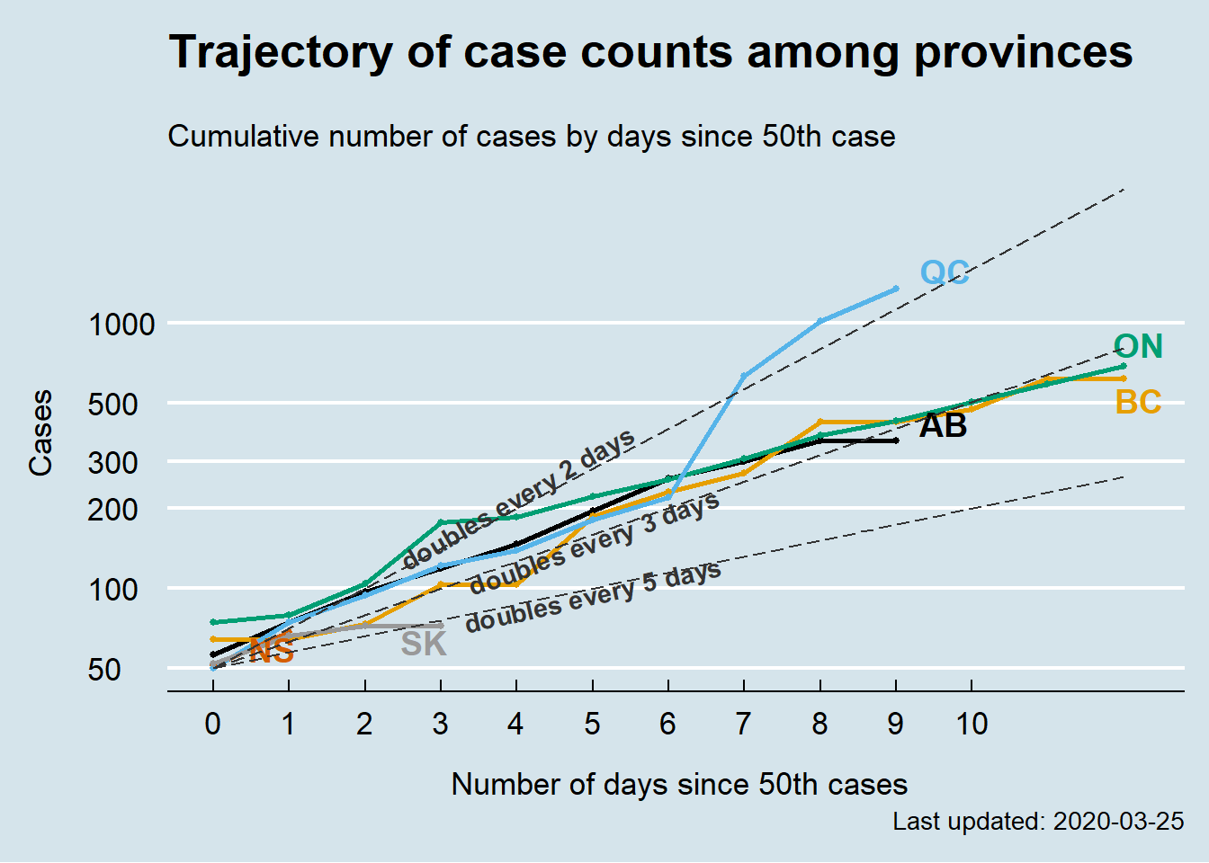On March 24th, Ontario, BC, and Alberta seem to be following the same exponential trajectory, with cases doubling almost every 3 days, while case numbers are growing faster in Quebec. It would be interesting to observe how this plot evovles in the coming days. A live version of the plot can be accessed here.

I created the case trajectory plot in R using ggplot2. I have copied the code below. Enjoy!

library(stringr)
library(tidyverse)
library(lubridate)
library(ggthemes)
library(scales)
library(RColorBrewer)
library(ggrepel)

caseType <- "Confirmed"
      caseType <- "confirmed_global"
      url <- paste0("https://raw.githubusercontent.com/CSSEGISandData/COVID-19/master/csse_covid_19_data/csse_covid_19_time_series/time_series_covid19_", caseType, ".csv")
      time_series_19_covid_Confirmed <- read_csv(url)
      
      covidCases <- time_series_19_covid_Confirmed %>% rename (country = "Country/Region") %>% rename (name = "Province/State") %>%
        filter (country == "Canada") 
      
      
       colourBlindPal <- c("#000000","#E69F00", "#D55E00", "#009E73", "#56B4E9", "#999999", "#CC79A7", "#0072B2")        

      lineDataCases <- covidCases %>% 
        select (-c(country, Lat, Long)) %>% 
        mutate(name = replace(name, name == "British Columbia", "BC")) %>% 
        mutate(name = replace(name, name == "Ontario", "ON")) %>% 
        mutate(name = replace(name, name == "Alberta", "AB")) %>% 
        mutate(name = replace(name, name == "Saskatchewan", "SK")) %>% 
        mutate(name = replace(name, name == "Manitoba", "MB")) %>% 
        mutate(name = replace(name, name == "Quebec", "QC")) %>% 
        mutate(name = replace(name, name == "Nova Scotia", "NS")) %>% 
        mutate(name = replace(name, name == "New Brunswick", "NB")) %>% 
        mutate(name = replace(name, name == "Newfoundland and Labrador", "NL"))%>%
        mutate(name = replace(name, name == "Prince Edward Island", "PE")) %>% 
        mutate(name = replace(name, name == "Yukon", "YT")) %>% 
        mutate(name = replace(name, name == "Northwest Territories", "NT")) %>% 
        mutate(name = replace(name, name == "Nunavut", "NU")) %>% 
        
        pivot_longer(cols = -1, names_to = "date", values_to = "Cases") %>%  mutate(date=mdy(date)) %>%
        filter (Cases>=50) %>% arrange (name, date) %>% 
        group_by(name) %>% mutate(date = date - date[1L]) %>%
        mutate(days = as.numeric(date)) #%>% filter(days <30)
      
    lastDay <- max(lineDataCases$days)  
    ggplot(data = lineDataCases, aes(x=days, y=Cases, colour = name)) +
  geom_line(size=0.9) + geom_point(size=1) + xlab ("\n Number of days since 50th cases") + 
  ylab ("Cases \n") +
  geom_text_repel(data = lineDataCases %>% 
              filter(days == last(days)), aes(label = name, 
                                              x = days + 0.2, 
                                              y = Cases, 
                                              color = name,
                                              fontface=2), size = 5) + 
  scale_y_continuous(trans = log10_trans(),
                     breaks = c(20, 50, 100, 200, 300, 500, 1000)) +
  scale_x_continuous(breaks = c(0:10)) +
  
  annotate("segment", linetype = "longdash", 
           x = 0, xend = lastDay, y = 50, yend = 50*(2^(1/3))^lastDay,
           colour = "#333333") +
  
  annotate(geom = "text", x = 5, y = 150, 
           label = "doubles every 3 days", color = "#333333", fontface=2,
           angle = 20) +
  
  
  annotate("segment", linetype = "longdash", 
           x = 0, xend = lastDay, y = 50, yend = 50*(2^(1/5))^lastDay,
           colour = "#333333") +
  annotate(geom = "text", x = 5, y = 95, 
           label = "doubles every 5 days", color = "#333333", fontface=2,
           angle = 13) +
  
  annotate("segment", linetype = "longdash", 
           x = 0, xend = lastDay, y = 50, yend = 50*(2^(1/2))^lastDay,
           colour = "#333333") +
  annotate(geom = "text", x = 4, y = 220, 
           label = "doubles every 2 days", color = "#333333", fontface=2,
           angle = 30) +
  
  scale_colour_manual(values=colourBlindPal) +
  theme_economist() + 
  ggtitle("Trajectory of case counts among provinces\n", subtitle = "Cumulative number of cases by days since 50th case") +
  theme(text = element_text(size=13)) +
  theme(legend.position = "none") +
  theme(legend.title=element_blank()) +
  labs(caption = paste0("Last updated: ", ymd(mdy(colnames(covidCases[length(covidCases)])))))